
Force Byte
Knowledge and Techniques
of Data Input in Excel (9)
0 Photo
We can call contiguous cells in an Excel worksheet to be a "range" and also name it, so that we can use these names to represent their respective ranges to facilitate setting formulas later. When naming a range, we should use an easy-to-remember name, e.g. the row or column label.
Defining a Range Name
To define the range name for cells D2:D3 as "Blackmail"
1. Select cells D2:D3.
2. Click the "Name Box" on the left of the formula bar and input "Blackmail" (See the figure below).
Quick Selection of a Range by its Name
We learn from the above that each range name represents a particular range. Therefore, choosing a name from the "Name Box" means selecting the range represented by that name.
To select D2:D3 by choosing its name "Blackmail"
1.Press the "(" button next to the "Name Box" and choose "Blackmail" (See the result in the figure below).
To find out in which year there is the highest number of blackmail using the concept of range name
1. Select cell D4.
2. Press the "Paste Function" button.
3.Choose "Most Recently Used" in the "Function category" field.
4.Choose "MAX" in the "Function name" field.
5.Press the "OK" button and drag the "MAX" box until it does not block the main window screen.
6.Input "Blackmail" into the "Number1" field (See the figure below).
For the sake of convenience, we can define multiple range names at the same time. We will use the column label to define the range name for a column of cells or the row label to define the range name for a row of cells.
In this example for defining multiple range names at the same time, the ranges will eventually be named as follows:
1. Select cells A1:F3, in which the column and row labels are included.
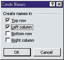
2. Select the "Create..." command of the "Name" option in the "Insert" menu.
3. Select "Top row" and "Left column" in the "Create Name" dialogue box (See the figure below).
To check the result of the above illustration, press the "(" button next to the "Name Box", and you will see the range names you have just created.
Next time, we will look at the basic techniques of copying formulas.
"Sharing IT as it applies to your daily life."
(E-mail address: ITB_ForceByte_Editor@police.gov.hk)
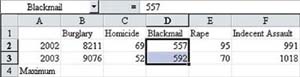
3. Press <Enter> and the cell range D2:D3 will be named as "Blackmail".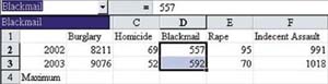
Application of Range Names in Formulas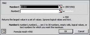
7. Press the "OK" button to close the box and let the calculated result display in cell D4 (See the figure below).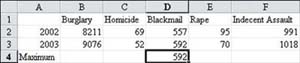
Defining Multiple Range Names at the Same Time
Burglary
B2:B3
Homicide
C2:C3
Blackmail
D2:D3
Rape
E2:E3
Indecent Assault
F2:F3
2002
B2:F2
2003
B3:F3
4.Press the "OK" button.