
Force Byte
Knowledge and Techniques
of Data Input in Excel (13)
0 Photo
In addition to common mathematical operators (e.g. "+", "-", "*", "/", "%", "^"), you can include the following "relational operators" in your Excel formulas.
> greater than
< smaller than
>= greater than or equal to
<= smaller than or equal to
<> not equal to
If the result of the comparison is true, Excel will return "TRUE"; otherwise it will return "FALSE".
Moreover, if there are more than one operators in a formula, Excel will execute them in the following order.
% (percentage)
^ (power)
* and / (multiplication and division)
+ and - (addition and subtraction)
= < > >= <= <> (relational operation)
(Order of execution starts from the top)
Just like ordinary mathematics, you may use parenthesis "( )" to alter the order of execution.
Later I will demonstrate the use of "relational operators" in formulas with a real example. In the meantime, I would like to introduce the "syntax" and "purpose" of the "COUNTIF" function.
Syntax: COUNTIF(range, "criteria")
Purpose: It is to count the number of cells within a particular range that meet the given "criteria".
For example, if you want to find out the number of cells that contain a value less than "60" within the range "C2:C3" from the example of the previous episode, the corresponding formula to be used should be "COUNTIF(C2:C3"<60")". When it is formally inputted into the cell, an "equal sign" should also be added to its left to make it become "=COUNTIF(C2:C3"<60")".
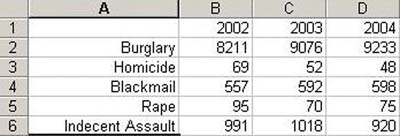
Now suppose we define "Common Crime" to be any types of crimes that have over 560 cases in a year, let's use a formula with "relational operators" to count from the following worksheet the types of crimes that meet this criteria in 2002, 2003 and 2004 respectively:
2. Input "Total of 'Common Crime'".
3. Press the <TAB>key and B7 will become the "active cell".
4. Input "=COUNTIF(B2:B6, ">560")" in B7. This formula will find out the number of cells within the range B2:B6 that contain a value over 560.
6. Move the mouse to the fill handle at the bottom right corner of cell B7. Now the cursor will become a "cross".
7. Drag the fill handle all the way through the range C7:D7. Cancel the range previously selected and you will get the following results.
"Sharing IT as it applies to your daily life."
(E-mail address: ISW_ForceByte_Editor@police.gov.hk)
= equal to
- (negative number)
1. Click A7.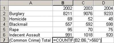
5. Press the <TAB> key. Now C7 becomes the "active cell". Then press the "(" key to make B7 become the "active cell" again.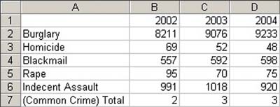
Up to here, I believe that you have a general idea of the application of "relational operators" to formulas. Next time, I will talk about how to sort data in Excel.